One of the oldest problems to have been solved using the calculus of variations was to find the equation for the shape formed by a hanging chain or flexible cord. Most often it is said that Galileo was the first to pose the problem and that he claimed that the resulting curve was a parabola. (See, for example, Goldstine [5], p. 32, footnote 42, and Truesdell [18], pp. 43–44.) Both of these statements are at best half true. Galileo’s exact words (in a classic English translation of his book Two New Sciences [4], p. 290) are
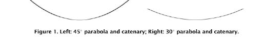
…a cord stretched more or less tightly assumes a curve which closely approximates the parabola....the coincidence is more exact in proportion as the parabola is drawn with less curvature or, so to speak, more stretched; so that using parabolas described with elevations less than 45° the chain fits its parabola almost perfectly….
Nowhere, to my knowledge, does Galileo address the question of finding the exact shape of the curve formed by the hanging chain. And he is exactly right that for a parabola with elevation less than 45° the curve formed by the chain is an extremely close approximation to the parabola (see Figures 1-2).
This passage follows immediately after an extended discussion during which Galileo presents one of his most famous discoveries: that the path of a projectile in a vacuum under the influence of gravity is a parabola ([4], pp. 244–290). In the course of the discussion, he points out that for a fixed initial velocity, the range will be maximized by an initial elevation of 45°. Finally, he addresses the question of how to quickly draw a number of parabolas, leading to the passage cited above.
The reason that one might mistake Galileo’s intentions and conclusions is that elsewhere in Two New Sciences ([4], p. 149) Galileo addresses the same problem and says simply that the “chain will assume the form of a parabola.” The reason that virtually everyone refers to this passage rather than the one in which Galileo spells out his conclusions in far greater detail and complete accuracy is not as clear.
Some of Galileo’s earliest experiments with hanging chains apparently date from the summer of 1602, when he was working with Guidobaldo del Monte. Had he thought to pose and try to answer the question of the exact equation for the shape of a hanging chain, he would have encountered two serious obstacles. First, the essential tool needed— the calculus—had not yet been invented. Second, the equation for the curve involves logarithms, which had also not yet been invented.
After the problem was finally explicitly stated, it was treated frequently by a number of authors between 1690 and 1720 and the correct answer derived, although some of the initial reasoning used was decidedly suspect. The curve became known as a catenary. Its equation is y = cosh x, the hyperbolic cosine, up to change of coordinates.
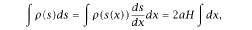
One method used to arrive at this result was the calculus of variations, finding the shape of a curve whose center of gravity is the lowest among all curves having a prescribed length and prescribed endpoints.
THE GATEWAY ARCH
It was Robert Hooke who in 1675 made the connection between the ideal shape of an arch and that of a hanging chain in an aphorism that says, in abbreviated form, “As hangs the chain, so stands the arch.” In other words, the geometry of a standing arch should mirror that of a hanging chain. The horizontal and vertical forces in a hanging chain must add to a force directed along the chain, since any component perpendicular to the chain would cause it to move in that direction to gain equilibrium. Similarly, one wants the combined forces at each point of an arch to add up to a vector tangent to the arch. In both cases, the horizontal component of the force is constant and simply transmitted along the arch or chain, while the vertical forces are mirror images.
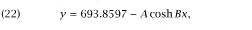
At least in part for these reasons, the shape of the Gateway Arch is often described mistakenly as a catenary (when not even more mistakenly as a parabola). In fact, the equation on which the arch is based is
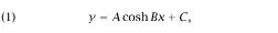
which is a catenary only if A = 1/B. For the Gateway Arch, A, B, and C are numerical constants, with A approximately equal to .69(1/B). As a result, those who wish to be more accurate describe the shape of the Arch as a “modified catenary” or, more often, a “weighted catenary.” The idea of the weighted catenary is to use either a chain with literal weights attached at various points or else a continuous version, such as a cord of varying density. (Both of those methods, incidentally, were used by Saarinen to find a shape for the Gateway Arch that appealed to him esthetically.)
Some natural questions to ask are
1. Is there a density function that yields the curve defined in equation (1) above, and if so, what is that function?
2. How descriptive is the term “weighted catenary?” In other words, what are the curves that fall in this category?
In order to answer these questions, we start with some precise definitions.
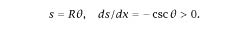
Definitions. (1) • A weighted chain C is a pair (f (x), ρ(s)) where f(x) is a suitably smooth function on an interval x1 ≤ x ≤ x2, s is arclength along the curve y = f(x), and ρ(s) is a positive continuous function of s.
• The function ρ(s) is called the density function of C.
• A weighted catenary is a weighted chain C in which
(i) −∞ <f ′(x1) < 0 <f ′(x2) < ∞,
(ii) f ′ ′(x) is continuous and positive,
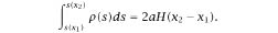
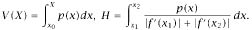
(iii) for x1 ≤ X ≤ x2,
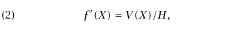
with
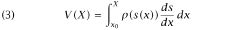
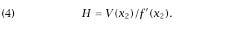
where f ′(x0) = 0, and H is a constant that depends on both f and ρ:
There is a certain amount of arbitrariness in these definitions. The smoothness of the function f(x) is deliberately left vague, since one might well want to allow different classes of functions in different situations. Similarly, one could allow the density function to have point masses or to be even more general.
Nonetheless, conditions (i)–(iii) are natural ones based on the physics underlying the problem. As noted earlier, for equilibrium we want the sum of the horizontal and vertical forces acting on the chain to be a vector tangent to the curve. The horizontal force is constant and simply transmitted along the curve, while the vertical force is due to gravity acting on the part of the chain from the lowest point to the point that we are considering on the curve and is equal to the total weight of that part of the chain.
Note that we do not require that the endpoints be at the same height—in other words, that f(x1) = f(x2)—although that will be true in all the examples of interest to us. In that case, condition (i) would follow from the physics of the situation. However, condition (i) does guarantee the existence of an interior point x0 of the interval where f ′ = 0, while condition (ii) implies that there is a unique such point.
Note also that the fact that there is a constant nonzero horizontal component to the force acting on the curve implies that the slope cannot be infinite at the endpoints. For example, a weighted catenary cannot be in the form of a semicircle.
Note finally that if ρ(s) is multiplied by a positive constant, then both H and V (x) are multiplied by the same constant. It follows that if the pair (f (x), ρ(s)) defines a weighted catenary, then so does the pair (f (x), cρ(s)) for any positive constant c.
We are now able to state our first result.
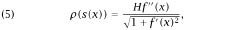
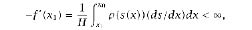
Theorem 1. If f (x) satisfies conditions (i) and (ii) above, then there is a function ρ(s), unique up to a multiplicative constant, such that the pair (f (x), ρ(s)) is a weighted catenary. Namely
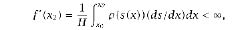
where H is an arbitrary positive constant. The value
of H is then given by
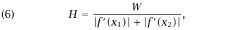
with
equal to the total weight of the chain.
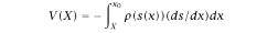
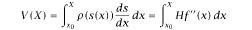
Proof. Suppose first that there exists a function ρ(s) such that the pair (f (x), ρ(s)) is a weighted catenary. Then by equations (2) and (3), for X ≥ x0,
Since ds/dx = √(1 + f ′(x)2), it follows that ρ(s) must have the form given in equation (5). For X < x0,
and
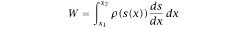
as before. Finally, the total weight W is
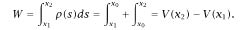
But V(x2) = Hf ′(x2) > 0, and V (x1) = Hf ′(x1) < 0, so that H takes the form indicated.
This proves that the density function ρ is uniquely determined by the function f (x) up to the choice of the constant H.
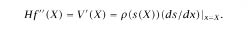
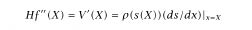
For the existence of a suitable density function ρ(s), given f(x), define ρ(s) by equation (5). Then
so that the pair (f (x), ρ(s)) form a weighted catenary, and then the constant H must have the form indicated in equation (6).
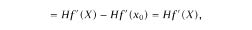
Example 1 (catenary).
Then
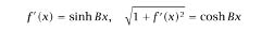
and f ′′(x) = B cosh Bx, so
Comment: This is a kind of inverse to the original catenary problem of asking for the shape taken by a uniformly weighted hanging chain. It tells us that only for a uniform chain will the resulting curve be a catenary.
Example 2 (parabola).
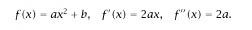
Then
and
and
Comment: This is in a sense the answer to Galileo’s original question of finding a mechanical method for drawing a parabola. It tells us exactly how we have to weight a chain so that it will hang in the form of a parabola. The key is that the weight distribution has to be uniform in the horizontal direction. For this reason, it is usually stated that the cables on a suspension bridge will hang in the shape of a parabola, since the weight of the cables themselves, together with that of the vertical support cables holding up the roadway, is small compared to the weight of the roadway, which has (in essence) a uniform horizontal weight distribution.
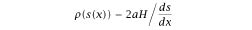
A curious by-product of the equation for the density ρ in the case of a parabola is that, since ds/dx ≥ 1, with equality only where f ′(x) = 0, it follows that ρ (s(x)) is maximum at the vertex and then decreases monotonically as | f ′(x)| increases. In other words, the chain has to be weighted the most near the vertex and then decrease as the steepness of the curve increases. As a result, if Saarinen had decided that he found a parabolic arch most pleasing esthetically, he would have been faced with the paradox that in order to have the line of thrust be everywhere directed along the arch, the arch would have to be thickest at the top and taper down toward the bottom, which would be both ungainly esthetically and potentially disastrous structurally.
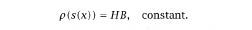
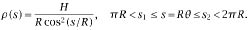
Example 3 (circular arc).
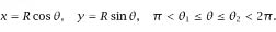
Then
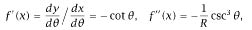
while
So
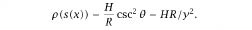
Comment: As noted earlier, a full semicircle cannot be a weighted catenary. We see explicitly that the density function would tend to infinity. However, any circular arc that is short of a semicircle at both ends can be realized (at least in theory) as a weighted catenary. The weighting is simply
Although this example may seem a typical “textbook example,” of no practical interest but merely a case that can be worked out explicitly, the opposite is true. A monumental “Gateway Arch” had been proposed as an entryway to a planned 1942 International Exposition in Rome, but it was derailed by the war. The arch was to be in the form of a semicircle, and the question of exactly how much it should be tapered was potentially critical (see [12] for more on this subject).
Note that this theorem answers the first part of Question 1 above about the existence of a density function yielding the particular “weighted catenary” shape of the Gateway Arch. It also answers Question 2 concerning the term “weighted catenary” itself, which turns out to have essentially no content beyond “convex curve.” Before turning to the second part of Question 1 regarding the exact form of the density function that yields the curve underlying the Gateway Arch, we prove a strong form of the converse to the theorem.
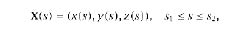
Converse of Theorem 1. Let C be a curve with endpoints P1 =(x1,y1,0) and P2 =(x2,y2,0), where x1 < x2. Assume that C is parameterized by arc length s in the form X(s)=(x(s), y(s), z(s)), P1=X(s1), P2 =X(s2).
Let ρ(s) > 0 be a continuous function along C, taken as a density function. Assume gravity acts in the negative y-direction and the pair (C,ρ(s)) is in equilibrium. Then
1. C lies entirely in the x, y -plane;
2. C is in the form of a graph y = f(x), x1 ≤ x ≤ x2;
3. f ′ (x) is finite and monotone increasing for x1 ≤ x ≤ x2.
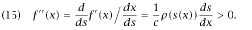
The idea underlying the proof is that if we know that C is a graph and (C,ρ(s)) is in equilibrium, so that equation (2) above holds, where V(X) is defined by (3), then
and for x1 ≤ x3 < x4 ≤ x2,
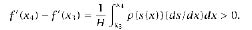
Hence condition 3 in the statement of the converse must hold.
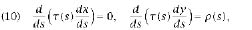
In terms of the representation above for C as X(s), the unit tangent vector to C will be given by T = dX/ds. We denote the tension at the point X(s) by τ, and for the case considered here, the tension vector will be
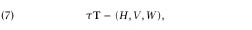
where H is constant and W = 0, while V is given by (3). Then
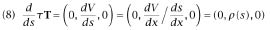
by (3), or
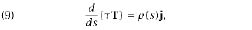
where j is the unit vector directed along the positive y-axis.
The proof of the above converse depends on the fact that equation (9) is the equation of equilibrium for an arbitrary curve joining the points P1, P2 in the x, y-plane, with no special assumptions about its shape (see [2], Chapter III, sections 1–3, for a detailed discussion of these questions in maximum generality. I would like to thank Joe Keller for providing this reference, as well as further helpful information. Note that in contrast to [2], we take the density ρ to mean weight, rather than mass, per unit length, so that the acceleration of gravity is absorbed into it).
Proof of the converse. Let C be defined by
where
Hence
where c and d are constants. We claim first that C must lie completely in the x, y-plane. If not, there must be a value s0, s1 < s0 < s2, where |z(s)| attains its maximum |z(s0)| > 0. Then (dz/ds)(s0) = 0, and the constant d in (13) must vanish. But if z(s) ̸≡ 0, there must be some value s3 such that dz/ds is nonzero at s3 and hence in an interval around s3. But then, since d = 0, it follows from (13) that τ(s) ≡ 0 on that interval. But that contradicts equation (9), since ρ(s) > 0. Hence we must have z(s) ≡ 0, and the curve lies entirely in the x, y-plane.
Exactly analogous reasoning using equation (11) shows that there cannot be a value s4 where dx/ds = 0. In fact, since x(s2) = x2 > x1 = x(s1), there must be a point where dx/ds > 0. It follows that dx/ds > 0 on the whole interval [s1, s2], and hence x is a strictly monotone increasing function of s on that interval. Thus, we have a monotone increasing inverse s(x), and we can set
defining C as a graph. It follows from equations (11) and (12) that
Hence f ′ (x) is a monotone increasing function of s and therefore of x. This completes the proof of the converse.
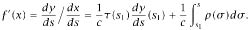
Note that it follows from the above that
Since c is the horizontal component of the tension vector, it is the quantity we denoted earlier by H, and equation (15) is the same as equation (5) above.
We now come to our principal example of the theorem.
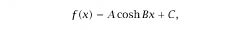
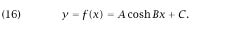
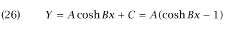
Definition 1. A flattened catenary is a curve of the form y = f (x)= A cosh Bx + C, or
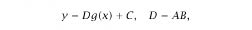
where 0 < D < 1, and
is a catenary.
Example 4 (flattened catenary). We examine this case in the following theorem.
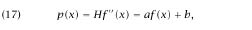
Theorem 2. Let C be a weighted catenary defined by the pair (f (x), ρ(s)), and let p(x) = ρ(s(x))(ds/dx). Assume that coordinates are chosen so that f ′ (0) = 0. Then p(x) will be of the form
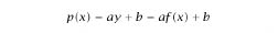
for some constants a > 0 and b if and only if f(x) is a flattened catenary
for constants A, B, C.
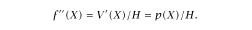
Proof. We have for all X in [x1, x2] that f ′(X) = V(X)/H, where
Then
Suppose first that
Then f ′(x) = AB sinh Bx and
Then
where
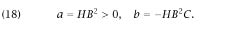
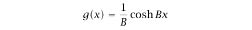
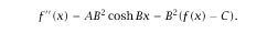
Conversely, suppose that p(x) = af (x) + b. Then f ′′(x) = (af (x) + b)/H. Let
Then g ′(0) = f ′(0) = 0, and
It follows that g(x) = A cosh Bx where B2 = a/H.
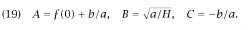
Hence
where
Historical Note
The flattened catenary was studied in the nineteenth century by a number of authors in France, England, Ireland, and Scotland. The first may have been Villarceau [19] (see Heyman [6], p. 48). Others include W. J. M. Rankine [13] and A. M. Howe [9]. (I thank William Thayer for these latter references and for alerting me to the connection between the equation for the Gateway Arch and the nineteenth century application discussed here.) In those works, the flattened catenary is often referred to as a “transformed catenary”, and the term “two-nosed catenary” is used for a highly flattened catenary, for reasons explained below. The context in which it arises is in answer to the question: What is the ideal shape of an arch that supports a horizontal roadway held up by evenly packed dirt on top of the arch? The vertical load applied to each point on the arch is then proportional to the distance from that point up to the level of the roadway. If we write the equation of the arch as y = f (x), where y is the distance from the roadway down to a given point on the arch, then the total vertical thrust acting on the part of the arch from the apex to an arbitrary point of the arch will correspond to the weight of a hanging chain from the minimum point to a given point, and it will be of the form ∫ p(x)dx, where p(x) is a linear function of y. The same reasoning as in the above theorem then shows that f (x) should be of the form (16): a flattened catenary (see, for example, Heyman [6], pp. 48-49).
We now come to the Gateway Arch itself. At first sight, it would appear to be a very different situation from that of an arch supporting a bridge, since it supports nothing except its own weight. On closer look, however, the fact that the Arch is tapered means that the weight supported at each level is not determined just by the length of the arch above it but by an integral with respect to arclength of a function exactly analogous to the density function for a weighted chain. The physical Gateway Arch is reasonably well modeled as one of a class of geometric shapes that are of interest in their own right.
Tube-like Domains
Two chance meetings in 1939 led to one of the major advances in differential geometry, the intrinsic proof by Chern of an n-dimensional Gauss–Bonnet theorem. The first occurred when mathematician Hermann Weyl attended a lecture by statistician Harold Hotelling in which Hotelling described a new result of his and posed an open question. Hotelling had been led by a statistical problem to pose the question: Given r > 0, what is the probability that a point chosen at random on the n-sphere would lie within a distance r of a given curve C? The answer amounts to computing the volume of the domain consisting of all points whose distance to C is less than r and comparing that to the total volume of the sphere. Hotelling was able to answer the question in both Euclidean n-space and the n-sphere for r sufficiently small [8]. The answer in Euclidean space was that the volume is equal to the length of C times the volume of an (n − 1)-ball of radius r, with an analogous result for the n-sphere. The answer was perhaps a surprise, since one might think that the volume of the “tube” around the curve C would depend somehow on the twists and turns in the curve, and not simply on its total length.
What Hotelling wanted to know, and was unable to derive, was a formula for the case that the curve C was replaced by a surface of two or more dimensions. Hermann Weyl [22] provided the answer in spectacular fashion: for a compact smooth submanifold S of Euclidean space, the volume of the domain consisting of all points lying within a fixed distance r of S is given, for r sufficiently small, by a polynomial in r whose coefficients are intrinsic quantities associated with S, and do not depend on the way that S is immersed in space. Most strikingly, the top coefficient does not even depend on the geometry of S, but only its topology; it is just a constant times the Euler characteristic χ of S.
The other chance meeting in 1939 took place between André Weil and Lars Ahlfors in Finland. Weil first learned about the classical Gauss–Bonnet theorem from Ahlfors, who expressed an interest in having a generalization to higher dimensions in order to develop a higher-dimensional Nevanlinna theory of value distribution ([20], p. 558, [21]). When Weil came to America several years later he met Carl Allendoerfer and learned that both Allendoerfer and Werner Fenchel had independently proved a Gauss–Bonnet theorem for manifolds embedded in Euclidean space, using Weyl’s formulas. Remembering Ahlfors’ desire for a general Gauss–Bonnet theorem, Weil was able, together with Allendoerfer, to prove the Gauss–Bonnet theorem for all Riemannian manifolds ([1], [20], p. 299). Their proof went via Weyl’s formulas together with local embedding theorems. Shortly after, using the appropriate form of the integrand from these earlier approaches, Chern was able to provide an intrinsic proof of the Gauss–Bonnet theorem without the detour through embeddings.
Our interest here is in a generalization of Hotelling’s result in a different direction. We go back to the case of a curve C in Euclidean space, but are interested in much more general domains.
Notation 1. A curve C in Rn will be denoted by
s = arc length parameter,
the unit tangent vector,
a positively oriented orthonormal frame field along C.
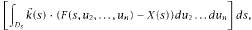
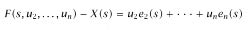
Definition 2. A tube-like domain T with centerline C is the image under a diffeomorphism F of a domain D in Rn, with coordinates u1,...,un, such that 0 < u1 < L, and for any t, 0 < t < L,the intersection Dt of D with the hyperplane u1 = t contains the point (t, 0,...,0). The map F satisfies F(u1, u2,...,un) = X(u1) + u2e2(u1) + ··· + unen(u1), with u1 = s = arc length parameter along C.
For 0 < s < L, let Ts be the intersection of T with the normal hyperplane to C at the point X(s). Then F : Ds → Ts is a linear transformation mapping Ds isometrically to Ts.
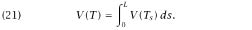
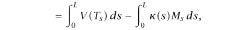
Theorem 3. Let T be a tube-like domain in Rn with centerline C. Then the volume V of T is given by
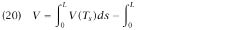
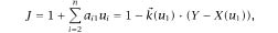
where k(s) = d2X/ds2 is the curvature vector, and for each fixed value of s, the vector
traces out the normal section Ts of T as the point (s, u2, . . . , un) ranges over the parameter domain Ds.
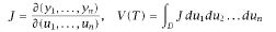
Proof. Let J = det dF be the Jacobian of the map F. If Y = (y1,...,yn) = F(u1,...,un), then
Now write
with ej = ej(u1), 0 ≤ u1 ≤ L. Then
and
Write
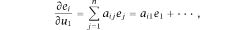
where the coefficients are given by
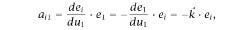
since the curvature vector equals .
So
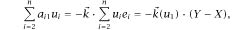
where aij = aij(u1), X = X(u1), Y = Y(u1,...,un).
Finally,
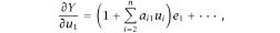
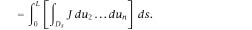
where the omitted terms involve the vectors e2, . . . , en, and will vanish after taking the wedge product with e2 through en. Hence,
as asserted.
Note. Different versions of this theorem have been known at least since 1978, when Michael Raugh [14] studied the case n = 3 in the context of the growth and structure of tendrils. Another discussion of the case n = 3 appears in Chapter 3 (Cálculo de várias variáveis) of [3], pp. 202–210. Both of those discussions assume the existence of a Frenet frame field for the centerline of the domain. A recent paper of Raugh [15] also treats the n-dimensional case.
Note. For the proof to be valid, one needs the Jacobian to be positive. If it were to change sign, then there would be cancellations, and the integral would not represent the actual volume. Since our definition of a tube-like domain includes the assumption that the defining map is a diffeomorphism, the Jacobian cannot change sign. However, if one starts with a domain D and tries to represent it as a tube domain, then one must check the positivity of the Jacobian. We shall return to this point later on.
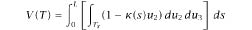
Corollary 1. If the point Xs is the centroid of Ts for each s ∈ [0, L], then
Note that it suffices to consider points where k(s)≠ 0.
Proof. For each value of s, the inner integral in the second term of the formula for V (T ) is a sum of terms consisting of integrals over Ds of terms of the form cjuj , where cj is a constant. But if X(s) is the centroid of Ts, then the origin is the centroid of Ds, and each of those integrals must vanish from the scenario.
Definition 3. Under the hypotheses of Corollary 1, the centerline C is called a centroid curve of T.
A given domain may have more than one centroid curve; for example, a Euclidean ball can be viewed as a tube-like domain with respect to any diameter as centerline, and that diameter will be a centroid curve for the ball.
Corollary 2 (Hotelling’s theorem). If T is a tube domain in Rn of radius r around a curve C of length L, then
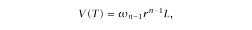
where ωk is the volume of the ball of radius r in Rk.
Proof. In this case D is a cylinder of radius r and height L. For 0 < s < L,the normal section Ts of T is an (n − 1)-ball of radius r centered at the point X(s) of C.
A number of statisticians returned to questions related to Hotelling’s theorem after a lapse of many years. See the paper [11] and further references given there.
Special Cases
n = 2. Then e2 is uniquely determined by e1 = dX/ds. The orthogonal section Ts is an interval Is, and the second term vanishes if X(s) is the midpoint of Is at all points where the curvature is nonzero.
Note. For n = 2, k(s) = κ(s)e2(s), where the curvature κ can be positive, negative, or zero.
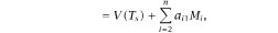
n = 3. If k(s) ≠ 0 at a point, then the same holds in an interval around the point, and we may define e2 = k(s)/κ(s), where κ(s) = |k(s)| is the curvature. Then e2 (s) is a smooth unit vector field on the interval, and e1, e2, together determine e3. Since de1/ds = k = κe2,we have a21 = −κ, a31 = 0, and J =1 − κ (s)u2. As already noted, this equation also holds whenever κ = 0. Therefore, for n = 3,
where Ms is the moment of Ts about the line through X(s) in the e3 (binormal) direction. It follows that for (21) to hold, one does not need X(s) to be the centroid of the orthogonal section, but only that the moment of that section be zero with respect to the line through X(s) in the binormal direction, at all points where κ ≠ 0. (See Raugh [15].)
An analogous statement holds for arbitrary n. Another formulation is
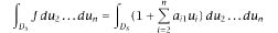
where Mi is the i-th moment of Ds, and ai1 = ai1(s).
Gateway Arch Specifications
The shape of the Gateway Arch is a polyhedral surface, the piecewise linear approximation by quadrilaterals to the surface S of the theoretical Gateway Arch, with two of the sides of each quadrilateral lying on designated straight-line segments of S.
Note. The surface just described is an abstract mathematical representation of the surface of the physical Gateway Arch, that surface consisting of the exterior of a set of stainless steel plates subject to a variety of distortions. Among those are the (uneven) expansion and contraction with changes of temperature, deflection due to wind forces, and deformation under the moving weight distribution of the internal transportation system carrying passengers to the top.
The theoretical Gateway Arch is a tube-like domain T whose centerline C is the reflection in a horizontal plane of a flattened catenary. The curve C is given by the equation
where A and B are the numerical constants
and x, y represent distances measured in feet. We may also write the equation of C as
where
represents the vertical distance down from the vertex of C.
The orthogonal section T (x, y) at the point (x, y) of C is in the form of an equilateral triangle of area Q(x,y), where the sides of T(x,y) when x = 0 (at the vertex of C) have length 17 feet and when y = 0 (at the base of the arch) have length 54 feet. The area Q(x, y) is defined by interpolating linearly in Y between the corresponding areas so defined:
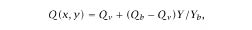
where Qv is the cross-sectional area at the vertex, and Qb is the corresponding area at the base. Since the area Q of an equilateral triangle is equal to
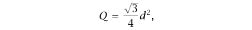
where d is the length of a side, and since d = 17 at the vertex v and d = 54 at the base, we find
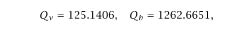
while Yb = Y|y=0 = 625.0925. It follows that
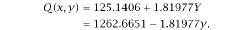
Using the relation above between the area Q and the side d of an equilateral triangle, we obtain the exact dimensions of the cross-sections at each height y. It remains to specify that the positions of the triangles in the planes orthogonal to the curve C are symmetric with respect to the x, y-plane, with one vertex lying in that plane and interior to the curve C, and that the centroid of each of those triangles lies on C, so that C is a centroid curve of the Arch.
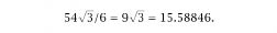
It follows from these specifications that the surface of the theoretical Gateway Arch is the union of three surfaces: a pair of ruled surfaces that are symmetric images with respect to the x, y-plane and meet in a curve lying in the x, y-plane, called the intrados of the Arch, together with a cylindrical surface orthogonal to that plane: the extrados. The maximum height of the extrados occurs at the point directly above the vertex of C where x = 0 and y = yv = 625.0925. At this point the orthogonal plane is vertical, and the distance from the vertex of C to the base of the triangle is one third of the length of the median, or 17 √ 3/6 = 4.90748. Adding this to yv gives for the maximum height of the Arch h = 629.99998.
The width of the Arch is a bit more subtle. We take the points where y = 0 on the centroid curve C to represent ground level. At those points, x = 299.2239 and −299.2239 so that the width of the curve at ground level is 598.4478. The equilateral triangle representing the cross-section at those points has side 54, and hence the distance to the outer curve of the Arch is
Adding this on each side to the width of C at ground level gives a total width for the Arch of 629.6247. However, since the curve C, although steep, is not vertical at ground level, the cross-section of the Arch is not horizontal, and the actual outer width is slightly larger. However, one sees that the dimensions of the centroid curve together with the size and shape of the cross-sections produce an arch that for all practical purposes has exactly the same total height as width. It may be worth noting, however, since it is sometimes a source of confusion, that the centroid curve is distinctly taller than wide, and the same is even more true of the inner curve of the Arch, whose height is 615.3 feet, and width is 536.1. For more on this and related matters, see [12].
Curvature Computations
Let y = f(x) = A cosh Bx = D(1/B cosh Bx) define a flattened catenary, where A, B are positive constants, and D = AB. Then f ′′(x) = B2y > 0 so that f is convex and the curvature κ > 0. Specifically,
For a catenary, D = 1 and κ = 1/By2,with a maximum of B at the vertex (0, 1/B) and decreasing monotonically to zero as y → ∞.
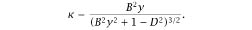
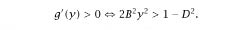
In general, let g(y) = (B2/κ)2 = B4R2, R = 1/κ. Then dR/dy ≥ 0 ⇔ g′ (y) ≥ 0. But one finds
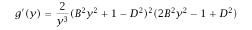
and since y ≥ A, B2y2 + 1 − D2 ≥ 1, and
Case 1: D > 1. An “elongated” catenary, obtained by stretching a catenary uniformly in the vertical direction. Then the right-hand side is negative, g′ (y) > 0 along the whole curve, so that R has a minimum and κ a maximum at the vertex, where x = 0, y = D/B, and κ = BD.
Case 2: D = 1. A catenary, for which, as we have seen, R has a minimum value of 1/B at the vertex and R → ∞ as y → ∞.
Case 3: 0 < D < 1. Then there are two possibilities.
Case 3a: D2 ≥ 1/3. Since y takes its minimum value A at the vertex, we have
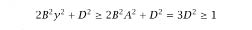
so that g′ (y) ≥ 0 along the whole curve, and as in cases 1 and 2, the curvature has its maximum value of BD at the vertex.
Case 3b: D2 < 1/3. Then 1 − D2 > 2D2 = 2B2A2, and we have g′ (y) < 0 in the interval
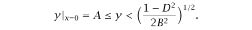
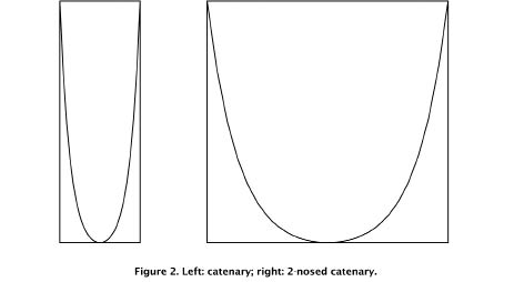
In this case, the vertex of the curve will be a local minimum of the curvature, which will increase monotonically until y reaches the value indicated on the right, where the curvature will reach its maximum. The curve is in this case sometimes referred to as a two-nosed catenary.
It is important to note that Figures 2-3 shows a two-nosed catenary for which D = 1/3, obtained by stretching a catenary uniformly in the horizontal direction by a factor of 3, which is equivalent, up to a similarity, to compressing it vertically by a factor of 3.
It may be worth observing that when illustrating geometric graphs, one often sees different scales used on the two axes. For a parabola, the resulting curve will still be a parabola, but for a catenary, the result will be a flattened or elongated catenary. As the figures, as well as the above calculation, makes clear, the shape may be very different geometrically from a true catenary. Such differences are obvious when different scales in the horizontal and vertical directions turn a circle into an ellipse, but they are often overlooked for noncompact curves such as the catenary.
Finally, we note that for the centroid curve of the Gateway Arch, we have D = AB = .69, well above the critical value D = √3/3 = .577..., so that the curvature will take its maximum value at the vertex, where it is equal to DB = .0069 so that the radius of curvature at that point is R = 145 feet, and it grows monotonically from there. Since all points of the cross-sectional equilateral triangles that define the Gateway Arch are less than 54 feet (and in fact, < 54√3/3 < 32 feet) from the centroid curve, it follows that the Jacobians entering into the computations leading up to equation (21) are all positive, where the Gateway Arch is considered as a tube-like domain.
Final Note
Although the essence of Hooke’s dictum relating the standing arch to the hanging chain seems clear, there are subtle issues that arise, some involving the fact that a standing arch is a three-dimensional body, whereas the hanging chain is modeled just as a curve. In fact, a careful analysis of the stability of an arch and its relation to the geometry of the arch is a subject about which whole books could be (and have been) written (see, for example, [6]).
Here is an example of a seemingly paradoxical fact that does not seem to have been mentioned anywhere. As we noted at the outset, the fact that the shape of a hanging chain is a catenary is often derived by using the calculus of variations, finding the curve of given length that has the lowest center of gravity. It follows then, according to Hooke, that the ideal shape of an arch would be an upside-down catenary, which would have the highest center of gravity among all arches of the same length. But that would appear to make it maximally unstable.